plot_c

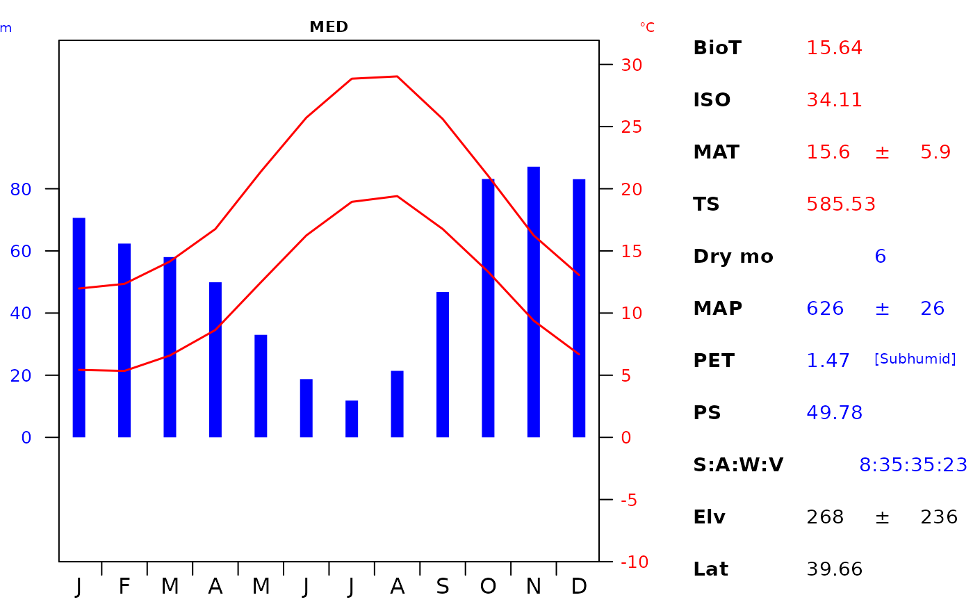
Creates a graph using the climate and elevation data which has been extracted for a given location. It accepts the data formatted from the ce_extract function.

plot_c(
  data,
  geo_id,
  interval_prec = 20,
  interval_temp = 5,
  stretch_temp = 4,
  p_cex = 1,
  nchr_main = 32,
  l_main = 0.1,
  l_prec = 0,
  l_month = -0.6,
  lwd_temp = 1.5,
  lwd_prec = 9,
  l_units = 0.1,
  l_tcols = c(14.5, 16.5, 18.5, 19.5, 22.5)
)

Arguments

data

List. Containing climate, elevation and latitude data sets. Structured by ce_extract().

geo_id

Character. Corresponding to a specific feature contained in the "location" argument (specifically in the "location_g" column).

interval_prec

Numeric. Interval of the precipitation axis.

interval_temp

Numeric. Interval of the temperature axis.

stretch_temp

Numeric. Ratio for stretching temperature relative to precipitation.

p_cex

Numeric. Text size for entire plot.

nchr_main

Numeric. Controls the number of characters of the main title before wrapping to a new line.

l_main

Numeric. Line position of the main title.

l_prec

Numeric. Line position of the y axis (precipitation).

l_month

Numeric. Line position of the x axis (months).

lwd_temp

Numeric. Line width of temperature.

lwd_prec

Numeric. Line width of precipitation.

l_units

Numeric. Line position of precipitation and temperature units.

l_tcols

List. Line position of the table columns. Must be length 5 corresponding to the position (left to right) for each column.

Value

Returns a base R family of plot. This function uses the dismo package to calculate isothermality (ISO), temperature seasonality (TS) and precipitation seasonality (PS).

References

Pizarro, M, Hernangómez, D. & Fernández-Avilés G. (2023). climaemet: Climate AEMET Tools. Comprehensive R Archive Network. doi:10.5281/zenodo.5205573

Walter, H.B., & Lieth, H. (1960). Klimadiagramm-Weltatlas. VEB Gustav Fischer Verlag, Jena.

See also

Download climate data: ce_download()

Author

James L. Tsakalos and Martin R. Smith

Examples

# Step 1. Import the Italian Biome polygon data
# Step 2. Run the download function
# Step 3. Run the extract function
#* See ce_download & ce_extract documentation

# Steps 1, 2 & 3 can be skipped by loading the extracted data (it_data)
data("it_data", package = "climenv")

# Step 4. Visualise the climatic envelope using our custom diagram

# first lets store the default graphics parameters
# we need to make some changes to ensure that the table fits in the plotting
# region.

# Set up plotting parameters
oldpar <- par(mar = c(1.5, 2.2, 1.5, 14) + 0.01)

plot_c(
  it_data, geo_id = "MED",
  l_tcols = c(14.5, 17, 18.5, 19.5, 21)
)


# Restore user options
par(oldpar)

# This output works if you export to a three column width sized image.